Tuning and diagnostics
1. Multi-threaded solving
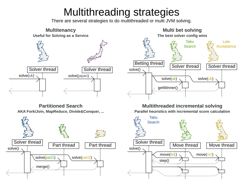
There are several ways of running the solver in parallel:
-
Multi-threaded incremental solving: Solve 1 dataset with multiple threads without sacrificing incremental score calculation.
-
Partitioned search: Split 1 dataset in multiple parts and solve them independently.
-
Multi bet solving: solve 1 dataset with multiple, isolated solvers and take the best result.
-
Not recommended: This is a marginal gain for a high cost of hardware resources.
-
Use the Benchmarker during development to determine the algorithm that is the most appropriate on average.
-
-
Multitenancy: solve different datasets in parallel.
-
The
SolverManagercan help with this.
-
1.1. Multi-threaded incremental solving
| This feature is exclusive to Timefold Solver Enterprise Edition. |
With this feature, the solver can run significantly faster, getting you the right solution earlier. It has been designed to speed up the solver in cases where move evaluation is the bottleneck. This typically happens when the constraints are computationally expensive, or when the dataset is large.
-
The sweet spot for this feature is when the move evaluation speed is up to 10 thousand per second. In this case, we have observed the algorithm to scale linearly with the number of move threads. Every additional move thread will bring a speedup, albeit with diminishing returns.
-
For move evaluation speeds on the order of 100 thousand per second, the algorithm no longer scales linearly, but using 4 to 8 move threads may still be beneficial.
-
For even higher move evaluation speeds, the feature does not bring any benefit. At these speeds, move evaluation is no longer the bottleneck. If the solver continues to underperform, perhaps you’re suffering from score traps or you may benefit from custom moves to help the solver escape local optima.
|
These guidelines are strongly dependent on move selector configuration, size of the dataset and performance of individual constraints. We recommend you benchmark your use case to determine the optimal number of move threads for your problem. |
1.1.1. Enabling multi-threaded incremental solving
Enable multi-threaded incremental solving
by adding a @PlanningId annotation
on every planning entity class and planning value class.
Then configure a moveThreadCount:
-
Service / Quarkus
-
Spring
-
Java
-
XML
Add the following to your application.properties:
quarkus.timefold.solver.move-thread-count=AUTOAdd the following to your application.properties:
timefold.solver.move-thread-count=AUTOUse the SolverConfig class:
SolverConfig solverConfig = new SolverConfig()
    ...
    .withMoveThreadCount("AUTO");
Add the following to your solverConfig.xml:
<solver xmlns="https://timefold.ai/xsd/solver" xmlns:xsi="http://www.w3.org/2001/XMLSchema-instance"
xsi:schemaLocation="https://timefold.ai/xsd/solver https://timefold.ai/xsd/solver/solver.xsd">

    ...
    <moveThreadCount>AUTO</moveThreadCount>
    ...

</solver>
Setting moveThreadCount to AUTO allows Timefold Solver to decide how many move threads to run in parallel.
This formula is based on experience and does not hog all CPU cores on a multi-core machine.
A moveThreadCount of 4 saturates almost 5 CPU cores.
The 4 move threads fill up 4 CPU cores completely
and the solver thread uses most of another CPU core.
The following moveThreadCounts are supported:
-
NONE(default): Don’t run any move threads. Use the single threaded code. -
AUTO: Let Timefold Solver decide how many move threads to run in parallel. On machines or containers with little or no CPUs, this falls back to the single threaded code. -
Static number: The number of move threads to run in parallel.
It is counter-effective to set a moveThreadCount
that is higher than the number of available CPU cores,
as that will slow down the move evaluation speed.
|
In cloud environments where resource use is billed by the hour, consider the trade-off between cost of the extra CPU cores needed and the time saved. Compute nodes with higher CPU core counts are typically more expensive to run and therefore you may end up paying more for the same result, even though the actual compute time needed will be less. |
|
Multi-threaded solving is still reproducible, as long as the resolved |
1.1.2. Advanced configuration
There are additional parameters you can supply to your solverConfig.xml:
<solver xmlns="https://timefold.ai/xsd/solver" xmlns:xsi="http://www.w3.org/2001/XMLSchema-instance"
    xsi:schemaLocation="https://timefold.ai/xsd/solver https://timefold.ai/xsd/solver/solver.xsd">
  <moveThreadCount>4</moveThreadCount>
  <threadFactoryClass>...MyAppServerThreadFactory</threadFactoryClass>
  ...
</solver>
To run in an environment that doesn’t like arbitrary thread creation,
use threadFactoryClass to plug in a custom thread factory.
1.2. Partitioned search
| This feature is exclusive to Timefold Solver Enterprise Edition. |
1.2.1. Algorithm description
It is often more efficient to partition large data sets (usually above 5000 planning entities) into smaller pieces and solve them separately. Partition Search is multi-threaded, so it provides a performance boost on multi-core machines due to higher CPU utilization. Additionally, even when only using one CPU, it finds an initial solution faster, because the search space sum of a partitioned Construction Heuristic is far less than its non-partitioned variant.
However, partitioning does lead to suboptimal results, even if the pieces are solved optimally, as shown below:
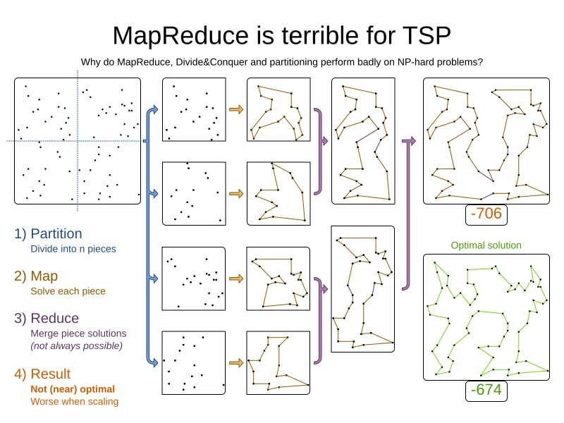
It effectively trades a short term gain in solution quality for long term loss. One way to compensate for this loss, is to run a non-partitioned Local Search after the Partitioned Search phase.
|
Not all use cases can be partitioned. Partitioning only works for use cases where the planning entities and value ranges can be split into n partitions, without any of the constraints crossing boundaries between partitions. |
1.2.2. Configuration
Simplest configuration:
  <partitionedSearch>
    <solutionPartitionerClass>...MyPartitioner</solutionPartitionerClass>
  </partitionedSearch>
Also add a @PlanningId annotation
on every planning entity class and planning value class.
There are several ways to partition a solution.
Advanced configuration:
  <partitionedSearch>
    ...
    <solutionPartitionerClass>...MyPartitioner</solutionPartitionerClass>
    <runnablePartThreadLimit>4</runnablePartThreadLimit>

    <constructionHeuristic>...</constructionHeuristic>
    <localSearch>...</localSearch>
  </partitionedSearch>
The runnablePartThreadLimit allows limiting CPU usage to avoid hanging your machine, see below.
To run in an environment that doesn’t like arbitrary thread creation, plug in a custom thread factory.
|
A logging level of |
Just like a <solver> element,
the <partitionedSearch> element can contain one or more phases.
Each of those phases will be run on each partition.
A common configuration is to first run a Partitioned Search phase (which includes a Construction Heuristic and a Local Search) followed by a non-partitioned Local Search phase:
  <partitionedSearch>
    <solutionPartitionerClass>...MyPartitioner</solutionPartitionerClass>

    <constructionHeuristic/>
    <localSearch>
      <termination>
        <diminishedReturns />
      </termination>
    </localSearch>
  </partitionedSearch>
  <localSearch/>
1.2.3. Partitioning a solution
Custom SolutionPartitioner
To use a custom SolutionPartitioner, configure one on the Partitioned Search phase:
  <partitionedSearch>
    <solutionPartitionerClass>...MyPartitioner</solutionPartitionerClass>
  </partitionedSearch>
Implement the SolutionPartitioner interface:
public interface SolutionPartitioner<Solution_> {

    List<Solution_> splitWorkingSolution(Solution_ workingSolution, Integer runnablePartThreadLimit);

}
The size() of the returned List is the partCount (the number of partitions).
This can be decided dynamically, for example, based on the size of the non-partitioned solution.
The partCount is unrelated to the runnablePartThreadLimit.
To configure values of a SolutionPartitioner dynamically in the solver configuration
(so the Benchmarker can tweak those parameters),
add the solutionPartitionerCustomProperties element and use custom properties:
  <partitionedSearch>
    <solutionPartitionerClass>...MyPartitioner</solutionPartitionerClass>
    <solutionPartitionerCustomProperties>
      <property name="myPartCount" value="8"/>
      <property name="myMinimumProcessListSize" value="100"/>
    </solutionPartitionerCustomProperties>
  </partitionedSearch>
1.2.4. Runnable part thread limit
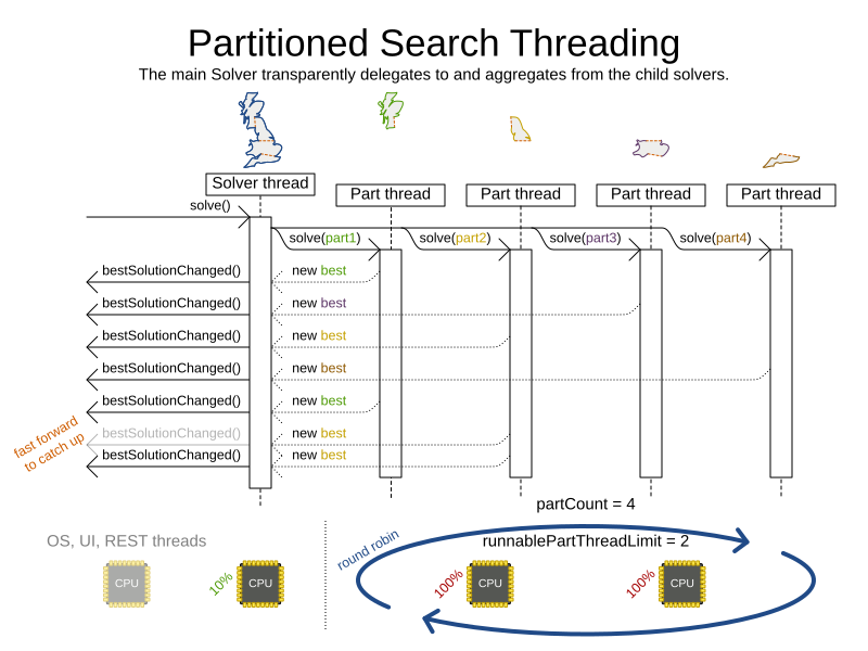
When running a multi-threaded solver, such as Partitioned Search, CPU power can quickly become a scarce resource, which can cause other processes or threads to hang or freeze. However, Timefold Solver has a system to prevent CPU starving of other processes (such as an SSH connection in production or your IDE in development) or other threads (such as the servlet threads that handle REST requests).
As explained in sizing hardware and software,
each solver (including each child solver) does no IO during solve() and therefore saturates one CPU core completely.
In Partitioned Search, every partition always has its own thread, called a part thread.
It is impossible for two partitions to share a thread,
because of asynchronous termination:
the second thread would never run.
Every part thread will try to consume one CPU core entirely, so if there are more partitions than CPU cores,
this will probably hang the system.
Thread.setPriority() is often too weak to solve this hogging problem, so another approach is used.
The runnablePartThreadLimit parameter specifies how many part threads are runnable at the same time.
The other part threads will temporarily block and therefore will not consume any CPU power.
This parameter basically specifies how many CPU cores are donated to Timefold Solver.
All part threads share the CPU cores in a round-robin manner
to consume (more or less) the same number of CPU cycles:
The following runnablePartThreadLimit options are supported:
-
UNLIMITED: Allow Timefold Solver to occupy all CPU cores, do not avoid hogging. Useful if a no hogging CPU policy is configured on the OS level. -
AUTO(default): Let Timefold Solver decide how many CPU cores to occupy. This formula is based on experience. It does not hog all CPU cores on a multi-core machine. -
Static number: The number of CPU cores to consume. For example:
<runnablePartThreadLimit>2</runnablePartThreadLimit>
|
If the |
1.3. Custom thread factory (WildFly, GAE, …)
The threadFactoryClass allows to plug in a custom ThreadFactory for environments
where arbitrary thread creation should be avoided,
such as most application servers (including WildFly) or Google App Engine.
Configure the ThreadFactory on the solver to create the move threads
and the Partition Search threads with it:
<solver xmlns="https://timefold.ai/xsd/solver" xmlns:xsi="http://www.w3.org/2001/XMLSchema-instance"
    xsi:schemaLocation="https://timefold.ai/xsd/solver https://timefold.ai/xsd/solver/solver.xsd">
  <threadFactoryClass>...MyAppServerThreadFactory</threadFactoryClass>
  ...
</solver>
2. Environment mode: are there bugs in my code?
The environment mode allows you to detect common bugs in your implementation. It does not affect the logging level.
You can set the environment mode:
-
Service / Quarkus
-
Spring Boot
-
Java
-
XML
Add the following to your application.properties:
quarkus.timefold.solver.environment-mode=STEP_ASSERTAdd the following to your application.properties:
timefold.solver.environment-mode=STEP_ASSERTSolverConfig solverConfig = new SolverConfig()
...
.withEnvironmentMode(EnvironmentMode.STEP_ASSERT);<solver xmlns="https://timefold.ai/xsd/solver" xmlns:xsi="http://www.w3.org/2001/XMLSchema-instance"
xsi:schemaLocation="https://timefold.ai/xsd/solver https://timefold.ai/xsd/solver/solver.xsd">
<environmentMode>STEP_ASSERT</environmentMode>
...
</solver>A solver has a single Random instance.
Some solver configurations use the Random instance a lot more than others.
For example, Simulated Annealing depends highly on random numbers, while Tabu Search only depends on it to deal with score ties.
The environment mode influences the seed of that Random instance.
2.1. Reproducibility
For the environment mode to be reproducible, any two runs of the same dataset with the same solver configuration must have the same result at every step. Choosing a reproducible environment mode enables you to reproduce bugs consistently. It also allows you to benchmark certain refactorings (such as a score constraint performance optimization) fairly across runs.
Regardless of whether the chosen environment mode itself is reproducible, your application might still not be fully reproducible because of:
-
Use of
HashSet(or anotherCollectionwhich has an undefined iteration order between JVM runs) for collections of planning entities or planning values (but not normal problem facts), especially in the solution implementation. Replace it with aSequencedSetorSequencedCollectionimplementation respectively, such asLinkedHashSetorArrayList.-
This also applies to
HashMap, which can be replaced by aSequencedMapimplementation such asLinkedHashMap.
-
-
Combining a time gradient-dependent algorithm (most notably Simulated Annealing) together with time spent termination. A large enough difference in allocated CPU time will influence the time gradient values. Replace Simulated Annealing with Late Acceptance, or replace time spent termination with step count termination.
2.2. Available environment modes
The following environment modes are available, in the order from least strict to most strict:
As the environment mode becomes stricter,
the solver becomes slower, but gains more error-detection capabilities.
STEP_ASSERT is already slow enough to prevent its use in production.
All modes other than NON_REPRODUCIBLE are reproducible.
2.2.1. TRACKED_FULL_ASSERT
The TRACKED_FULL_ASSERT mode turns on all the FULL_ASSERT assertions
and additionally tracks changes to the working solution.
This allows the solver to report exactly what variables were corrupted.
In particular, the solver will recalculate all shadow variables from scratch on the solution after the undo and then report:
-
Genuine and shadow variables that are different between "before" and "undo". After an undo move is evaluated, it is expected to exactly match the original working solution.
-
Variables that are different between "from scratch" and "before". This is to detect if the solution was corrupted before the move was evaluated due to shadow variable corruption.
-
Variables that are different between "from scratch" and "undo". This is to detect if recalculating the shadow variables from scratch is different from the incremental shadow variable calculation.
-
Missing variable events for the actual move. Any variable that changed between the "before move" solution and the "after move" solution without the solver being notified of the change.
-
Missing events for undo move. Any variable that changed between the "after move" solution and "after undo move" solution without the solver being notified of the change.
This mode is reproducible (see the reproducible mode).
It is also intrusive because it calls the method calculateScore() more frequently than a non-assert mode.
The TRACKED_FULL_ASSERT mode is by far the slowest mode,
because it clones solutions before and after each move.
2.2.2. FULL_ASSERT
The FULL_ASSERT mode turns on all assertions and will fail-fast on a bug in a Move implementation,
a constraint, the engine itself, …
It is also intrusive
because it calls the method calculateScore() more frequently than a NO_ASSERT mode,
making the FULL_ASSERT mode very slow.
This mode is reproducible.
This mode is neither better nor worse than NON_INTRUSIVE_FULL_ASSERT - each can catch different types of errors, on account of performing score calculations at different times.
|
2.2.3. NON_INTRUSIVE_FULL_ASSERT
The NON_INTRUSIVE_FULL_ASSERT mode turns on most assertions and will fail-fast on a bug in a Move implementation,
a constraint, the engine itself, …
It is not intrusive,
as it does not call the method calculateScore() more frequently than a NO_ASSERT mode.
This mode is reproducible. This mode is also very slow, on account of all the additional checks performed.
This mode is neither better nor worse than FULL_ASSERT - each can catch different types of errors, on account of performing score calculations at different times.
|
2.2.4. STEP_ASSERT
The STEP_ASSERT mode turns on most assertions (such as assert that an undoMove’s score is the same as before the Move)
to fail-fast on a bug in a Move implementation, a constraint, the engine itself, …
This makes it slow.
This mode is reproducible.
It is also intrusive because it calls the method calculateScore() more frequently than a non-assert mode.
We recommend that you write a test case that does a short run of your planning problem with the STEP_ASSERT mode on.
|
2.2.5. PHASE_ASSERT (default)
The PHASE_ASSERT is the default mode because it is recommended during development.
This mode is reproducible
and it gives you the benefit of quickly checking for score corruptions.
If you can guarantee that your code is and will remain bug-free,
you can switch to the NO_ASSERT mode for a marginal performance gain.
In practice, this mode disables certain concurrency optimizations, such as work stealing.
2.2.6. NO_ASSERT
The NO_ASSERT environment mode behaves in all aspects like the default PHASE_ASSERT mode,
except that it does not give you any protection against score corruption bugs.
As such, it can be negligibly faster.
2.2.7. NON_REPRODUCIBLE
This mode can be slightly faster than any of the other modes, but it is not reproducible. Avoid using it during development as it makes debugging and bug fixing painful. If your production environment doesn’t care about reproducibility, use this mode in production.
Unlike all the other modes, this mode doesn’t use any fixed random seed unless one is provided.
2.3. Best practices
There are several best practices to follow throughout the lifecycle of your application:
- In production
-
Use the
PHASE_ASSERTmode if you need reproducibility, otherwise useNON_REPRODUCIBLE. - In development
-
-
Use the
PHASE_ASSERTmode to catch bugs early. -
Write a test case that does a short run of your planning problem in
STEP_ASSERTmode. -
Have nightly builds that run for several minutes in
FULL_ASSERTandNON_INTRUSIVE_FULL_ASSERTmodes.
-
3. Logging level: what is the Solver doing?
The best way to illuminate the black box that is a Solver, is to play with the logging level:
-
error: Log errors, except those that are thrown to the calling code as a
RuntimeException.If an error happens, Timefold Solver normally fails fast: it throws a subclass of
RuntimeExceptionwith a detailed message to the calling code. It does not log it as an error itself to avoid duplicate log messages. Except if the calling code explicitly catches and eats thatRuntimeException, aThread's defaultExceptionHandlerwill log it as an error anyway. Meanwhile, the code is disrupted from doing further harm or obfuscating the error. -
warn: Log suspicious circumstances.
-
info: Log every phase and the solver itself. See scope overview.
-
debug: Log every step of every phase. See scope overview.
-
trace: Log every move of every step of every phase. See scope overview.
|
Turning on Even Both trace logging and debug logging cause congestion in multi-threaded solving with most appenders, see below. In Eclipse, |
For example, set it to debug logging, to see when the phases end and how fast steps are taken:
INFO  Solving started: time spent (31), best score (0hard/0soft), environment mode (PHASE_ASSERT), move thread count (NONE), random (JDK with seed 0).
INFO  Problem scale: entity count (4), variable count (8), approximate value count (4), approximate problem scale (256).
DEBUG     CH step (0), time spent (47), score (0hard/0soft), selected move count (4), picked move ([Math(0) {null -> Room A}, Math(0) {null -> MONDAY 08:30}]).
DEBUG     CH step (1), time spent (50), score (0hard/0soft), selected move count (4), picked move ([Physics(1) {null -> Room A}, Physics(1) {null -> MONDAY 09:30}]).
DEBUG     CH step (2), time spent (51), score (-1hard/-1soft), selected move count (4), picked move ([Chemistry(2) {null -> Room B}, Chemistry(2) {null -> MONDAY 08:30}]).
DEBUG     CH step (3), time spent (52), score (-2hard/-1soft), selected move count (4), picked move ([Biology(3) {null -> Room A}, Biology(3) {null -> MONDAY 08:30}]).
INFO  Construction Heuristic phase (0) ended: time spent (53), best score (-2hard/-1soft), move evaluation speed (1066/sec), step total (4).
DEBUG     LS step (0), time spent (56), score (-2hard/0soft), new best score (-2hard/0soft), accepted/selected move count (1/1), picked move (Chemistry(2) {Room B, MONDAY 08:30} <-> Physics(1) {Room A, MONDAY 09:30}).
DEBUG     LS step (1), time spent (60), score (-2hard/1soft), new best score (-2hard/1soft), accepted/selected move count (1/2), picked move (Math(0) {Room A, MONDAY 08:30} <-> Physics(1) {Room B, MONDAY 08:30}).
DEBUG     LS step (2), time spent (60), score (-2hard/0soft),     best score (-2hard/1soft), accepted/selected move count (1/1), picked move (Math(0) {Room B, MONDAY 08:30} <-> Physics(1) {Room A, MONDAY 08:30}).
...
INFO  Local Search phase (1) ended: time spent (100), best score (0hard/1soft), move evaluation speed (2021/sec), step total (59).
INFO  Solving ended: time spent (100), best score (0hard/1soft), move evaluation speed (1100/sec), phase total (2), environment mode (PHASE_ASSERT), move thread count (NONE).
All time spent values are in milliseconds.
-
Java
Everything is logged to SLF4J, which is a simple logging facade which delegates every log message to Logback, Apache Commons Logging, Log4j or java.util.logging. Add a dependency to the logging adaptor for your logging framework of choice.
If you are not using any logging framework yet, use Logback by adding this Maven dependency (there is no need to add an extra bridge dependency):
    <dependency>
      <groupId>ch.qos.logback</groupId>
      <artifactId>logback-classic</artifactId>
      <version>1.x</version>
    </dependency>
Configure the logging level on the ai.timefold.solver package in your logback.xml file:
<configuration>

  <logger name="ai.timefold.solver" level="debug"/>

  ...

</configuration>
If it isn’t picked up, temporarily add the system property -Dlogback.debug=true to figure out why.
|
When running multiple solvers or a multi-threaded solver,
most appenders (including the console) cause congestion with |
|
In a multitenant application, multiple Then configure your logger to use different files for each |
4. Monitoring the solver
Timefold Solver exposes metrics through Micrometer which you can use to monitor the solver.
- Service
-
Micrometer is automatically configured in the service module. See Exposing Metrics for setup instructions and the list of available metrics.
- Quarkus / Spring Boot
-
Timefold automatically connects to configured Micrometer registries in Quarkus and Spring Boot. Add the appropriate Micrometer registry dependency for your monitoring system.
- Java
-
When using plain Java, you must add the metrics registry to the global registry manually.
-
You have configured a Micrometer registry. For information about configuring Micrometer registries, see the Micrometer web site.
-
Add configuration information for the Micrometer registry for your desired monitoring system to the global registry.
-
Add the following line below the configuration information, where
<REGISTRY>is the name of the registry that you configured:Metrics.addRegistry(<REGISTRY>);The following example shows how to add the Prometheus registry:
PrometheusMeterRegistry prometheusRegistry = new PrometheusMeterRegistry(PrometheusConfig.DEFAULT);

try {
    HttpServer server = HttpServer.create(new InetSocketAddress(8080), 0);
    server.createContext("/prometheus", httpExchange -> {
        String response = prometheusRegistry.scrape(); (1)
        httpExchange.sendResponseHeaders(200, response.getBytes().length);
        try (OutputStream os = httpExchange.getResponseBody()) {
            os.write(response.getBytes());
        }
    });

    new Thread(server::start).start();
} catch (IOException e) {
    throw new RuntimeException(e);
}

Metrics.addRegistry(prometheusRegistry);
The following metrics are exposed:
+
|
The names and format of the metrics vary depending on the registry. |
+
* timefold.solver.errors.total: the total number of errors that occurred while solving since the start
of the measuring.
* timefold.solver.solve.duration.active-count: the number of solvers currently solving.
* timefold.solver.solve.duration.seconds-max: run time of the
longest-running currently active solver.
* timefold.solver.solve.duration.seconds-duration-sum: the sum of each active solver’s solve duration. For example, if there are two active solvers, one running for three minutes and the other for one minute, the total solve time is four minutes.
4.1. Additional metrics
For more detailed monitoring, Timefold Solver can be configured to monitor additional metrics at a performance cost.
<solver xmlns="https://timefold.ai/xsd/solver" xmlns:xsi="http://www.w3.org/2001/XMLSchema-instance"
    xsi:schemaLocation="https://timefold.ai/xsd/solver https://timefold.ai/xsd/solver/solver.xsd">
  <monitoring>
    <metric>BEST_SCORE</metric>
    <metric>SCORE_CALCULATION_COUNT</metric>
    ...
  </monitoring>
  ...
</solver>
The following metrics are available:
-
SOLVE_DURATION(default, Micrometer meter id: "timefold.solver.solve.duration"): Measurse the duration of solving for the longest active solver, the number of active solvers and the cumulative duration of all active solvers. -
ERROR_COUNT(default, Micrometer meter id: "timefold.solver.errors"): Measures the number of errors that occur while solving. -
SCORE_CALCULATION_COUNT(default, Micrometer meter id: "timefold.solver.score.calculation.count"): Measures the number of score calculations Timefold Solver performed. -
MOVE_EVALUATION_COUNT(default, Micrometer meter id: "timefold.solver.move.evaluation.count"): Measures the number of move evaluations Timefold Solver performed. -
PROBLEM_ENTITY_COUNT(default, Micrometer meter id: "timefold.solver.problem.entities"): Measures the number of entities in the problem submitted to Timefold Solver. -
PROBLEM_VARIABLE_COUNT(default, Micrometer meter id: "timefold.solver.problem.variables"): Measures the number of genuine variables in the problem submitted to Timefold Solver. -
PROBLEM_VALUE_COUNT(default, Micrometer meter id: "timefold.solver.problem.values"): Measures the approximate number of planning values in the problem submitted to Timefold Solver. -
PROBLEM_SIZE_LOG(default, Micrometer meter id: "timefold.solver.problem.size.log"): Measures the approximate log 10 of the search space size for the problem submitted to Timefold Solver. -
BEST_SCORE(Micrometer meter id: "timefold.solver.best.score.*"): Measures the score of the best solution Timefold Solver found so far. There are separate meters for each level of the score. For instance, for aHardSoftScore, there aretimefold.solver.best.score.hard.scoreandtimefold.solver.best.score.soft.scoremeters. -
STEP_SCORE(Micrometer meter id: "timefold.solver.step.score.*"): Measures the score of each step Timefold Solver takes. There are separate meters for each level of the score. For instance, for aHardSoftScore, there aretimefold.solver.step.score.hard.scoreandtimefold.solver.step.score.soft.scoremeters. -
BEST_SOLUTION_MUTATION(Micrometer meter id: "timefold.solver.best.solution.mutation"): Measures the number of changed planning variables between consecutive best solutions. -
MOVE_COUNT_PER_STEP(Micrometer meter id: "timefold.solver.step.move.count"): Measures the number of moves evaluated in a step. -
MOVE_COUNT_PER_TYPE(Micrometer meter id: "timefold.solver.move.type.count"): Measures the number of moves evaluated per move type. -
MEMORY_USE(Micrometer meter id: "jvm.memory.used"): Measures the amount of memory used across the JVM. This does not measure the amount of memory used by a solver; two solvers on the same JVM will report the same value for this metric. -
CONSTRAINT_MATCH_TOTAL_BEST_SCORE(Micrometer meter id: "timefold.solver.constraint.match.best.score.*"): Measures the score impact of each constraint on the best solution Timefold Solver found so far. There are separate meters for each level of the score, with tags for each constraint. For instance, for aHardSoftScorefor a constraint "Minimize Cost", there aretimefold.solver.constraint.match.best.score.hard.scoreandtimefold.solver.constraint.match.best.score.soft.scoremeters with a tag "constraint.id=Minimize Cost". -
CONSTRAINT_MATCH_TOTAL_STEP_SCORE(Micrometer meter id: "timefold.solver.constraint.match.step.score.*"): Measures the score impact of each constraint on the current step. There are separate meters for each level of the score, with tags for each constraint. For instance, for aHardSoftScorefor a constraint "Minimize Cost", there aretimefold.solver.constraint.match.step.score.hard.scoreandtimefold.solver.constraint.match.step.score.soft.scoremeters with a tag "constraint.id=Minimize Cost". -
PICKED_MOVE_TYPE_BEST_SCORE_DIFF(Micrometer meter id: "timefold.solver.move.type.best.score.diff.*"): Measures how much a particular move type improves the best solution. There are separate meters for each level of the score, with a tag for the move type. For instance, for aHardSoftScoreand aChangeMovefor the room of a lesson, there aretimefold.solver.move.type.best.score.diff.hard.scoreandtimefold.solver.move.type.best.score.diff.soft.scoremeters with the tagmove.type=ChangeMove(Lesson.room). -
PICKED_MOVE_TYPE_STEP_SCORE_DIFF(Micrometer meter id: "timefold.solver.move.type.step.score.diff.*"): Measures how much a particular move type improves the best solution. There are separate meters for each level of the score, with a tag for the move type. For instance, for aHardSoftScoreand aChangeMovefor the room of a lesson, there aretimefold.solver.move.type.step.score.diff.hard.scoreandtimefold.solver.move.type.step.score.diff.soft.scoremeters with the tagmove.type=ChangeMove(Lesson.room).
5. Random number generator
Many heuristics and metaheuristics depend on a pseudorandom number generator for move selection, to resolve score ties, probability based move acceptance, … During solving, the same RandomGenerator instance is reused to improve reproducibility, performance and uniform distribution of random values.
To change the random seed of that RandomGenerator instance, specify a randomSeed:
-
Service / Quarkus
-
Spring Boot
-
XML
quarkus.timefold.solver.random-seed=0timefold.solver.random-seed=0<solver xmlns="https://timefold.ai/xsd/solver" xmlns:xsi="http://www.w3.org/2001/XMLSchema-instance"
xsi:schemaLocation="https://timefold.ai/xsd/solver https://timefold.ai/xsd/solver/solver.xsd">
<randomSeed>0</randomSeed>
...
</solver>